Sparse-view photoacoustic reconstruction

Inverse problems · Imaging

My contribution

I built a synthetic sparse-view pipeline and compared calibrated time reversal, a U-Net refinement, exact-model Tikhonov inversion and an unrolled network, then tested sound-speed mismatch and training-prior shift, and designed and ran two preregistered experiments on the failure that the shift exposed: a training intervention and a factorial diagnostic of the trained networks.

Verified resultsCompleted synthetic study · two preregistered experiments reported

An unrolled network trained on four phantom families is 11 to 18 dB ahead of noise-matched Tikhonov on its sharp-edged training families, but behind it on unseen thin structures with 64 sensors. Two preregistered experiments followed: an intervention repaired one gap in the learned prior, and a factorial diagnostic found structural thinness the best-supported remaining factor, with curvature not supported as a cause and the role of edge profile unresolved. All data are synthetic.

View source code ↗All projects

Quantitative findings

Photoacoustic tomographyTikhonov inversionUnrolled networksDistribution shiftPreregistered experiments

Research question

Reconstructing the initial pressure distribution of an imaged structure from sparse-view photoacoustic sensor measurements, a PDE-governed acoustic inverse problem in which classical time-reversal reconstruction degrades into streak artefacts as the sensor array is undersampled. The study asks when a learned reconstruction is better than a model-based one, what that advantage depends on, and what explains its failures on images unlike the training set.

Methodology

A synthetic acoustic forward model (j-Wave) simulates PML-bounded wave propagation from seeded phantoms on a 64 × 64 grid to a sparse circular array of 16 or 64 sensors. Four reconstructions are compared: time reversal, amplitude-calibrated by one least-squares gain per sensor count; a U-Net that refines the time-reversal estimate; Tikhonov-regularised least squares through the forward simulator written as an explicit matrix; and an unrolled network that alternates a small CNN with exact Tikhonov data-consistency solves. Calibration gains and the Tikhonov weight are fitted on the training split only.

Experimental setup and verification

400 held-out test images and 5 independently trained networks per learned method, with 95% bootstrap intervals over images reported separately from the spread between networks. The Tikhonov matrix reproduces the simulator, and its adjoint, gradient and normal equations are tested. The protocols of the mismatch, unrolled and mixed-family experiments were fixed before their results were seen. The two follow-up experiments were preregistered: hypotheses, numerical thresholds and decision rules were committed to the repository before any network was trained or any test image reconstructed, and negative and unexpected outcomes are reported as they came.

Baselines and the inverse crime

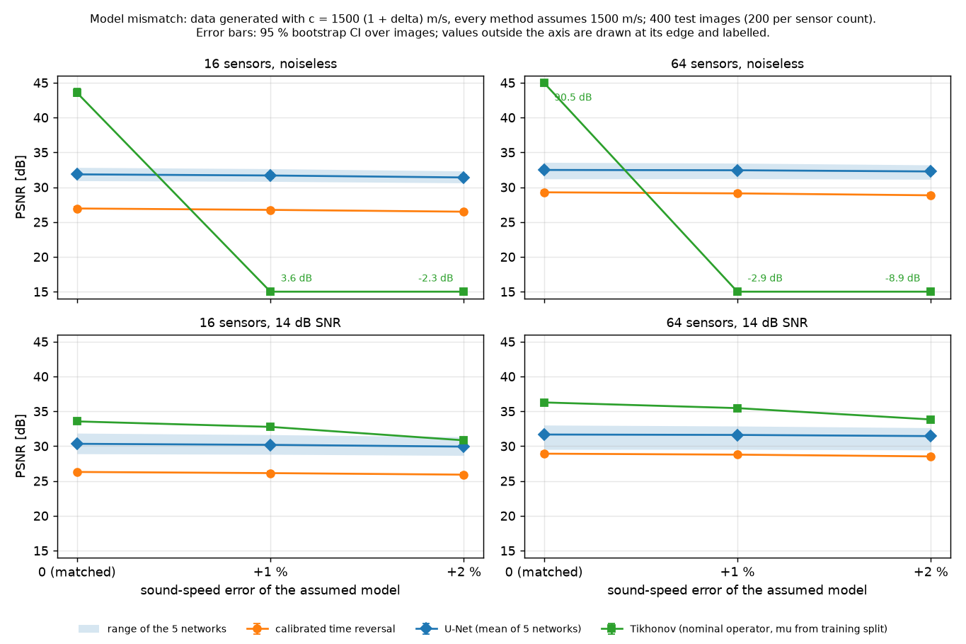
The U-Net improves PSNR over calibrated time reversal by 4.9 dB at 16 sensors and 3.2 dB at 64, with about 2 dB variation between identically trained networks. Tikhonov with the exact forward operator and a weight tuned for the known noise level scores higher than the average U-Net at every noise level, but this is an inverse crime: its noiseless values (43.6 and 90.5 dB) are near-exact inversion of data generated by the same operator, not expected reconstruction quality.

With the data generated at a sound speed 1 to 2% above the assumed value, Tikhonov tuned on noiseless data fails. At 14 dB SNR, with its weight tuned for that noise level, its PSNR lead over the U-Net shrinks to 0.9 to 3.9 dB. Time reversal and the U-Net change by under 0.5 dB.

Learned prior and its limits

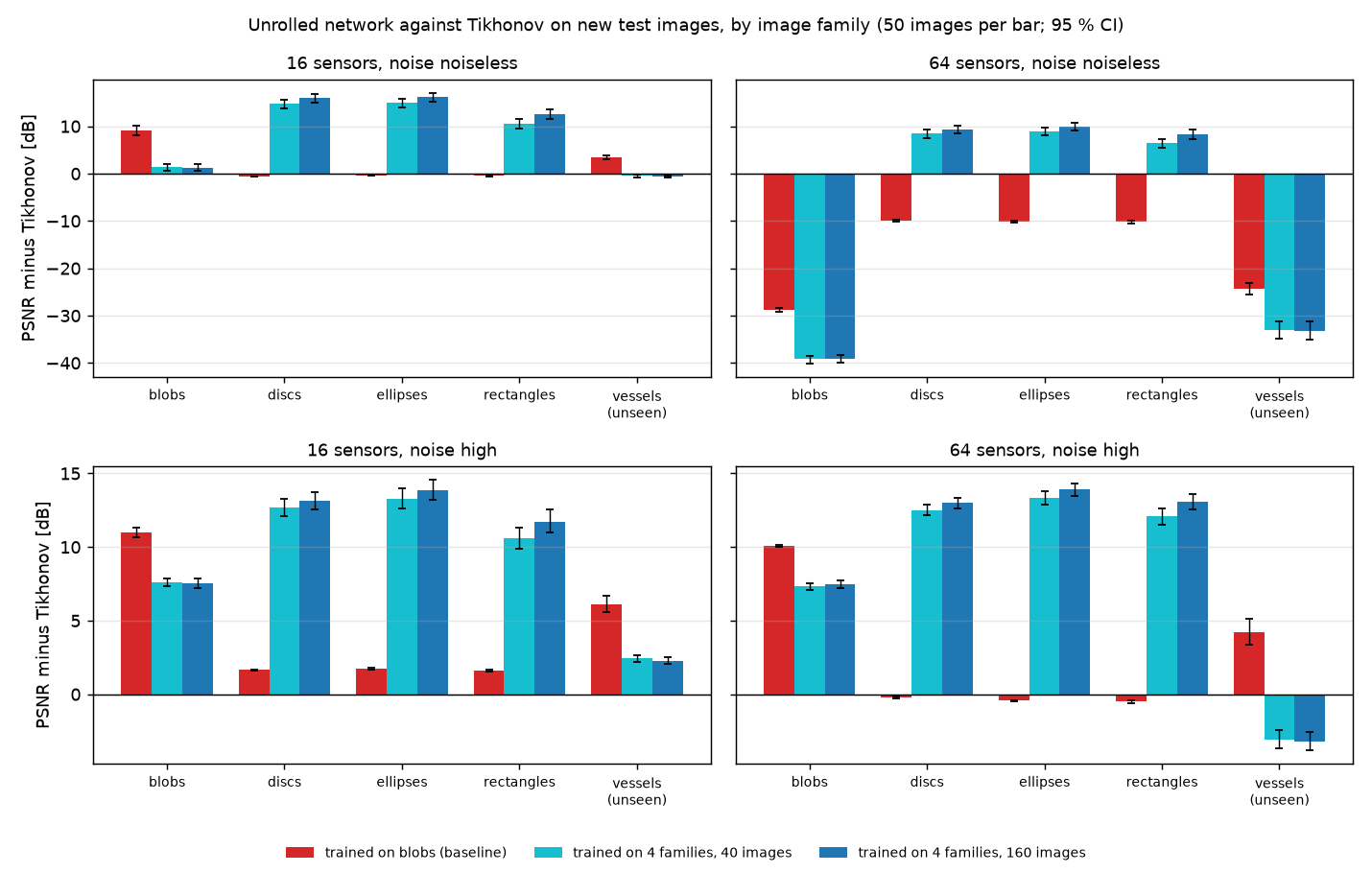
The unrolled network trained with noise is 8 to 15 dB ahead of noise-matched Tikhonov at every noise level on the blob test set, without being told the noise level; the exception is noiseless 64-sensor data, where Tikhonov inverts its own model exactly. That margin depends on the training images. On sharp-edged discs, which the network never saw, the lead is gone.

Training the same network on four phantom families together (blobs, discs, ellipses, rectangles) restores a large advantage on all four, at a cost of 2 to 4 dB on blobs under strong noise. The advantage does not transfer to an unseen family of thin vessel-like lines: at 14 dB SNR the mixed network is 2.3 dB ahead of Tikhonov with 16 sensors and 3.2 dB behind it with 64. Going from 16 to 64 sensors improves Tikhonov by 7.4 dB on these images and the network by 1.9 dB, so more sensors help the model-based method more than a network whose prior does not fit the image.

+11 to +18 dBMixed network vs. Tikhonov, trained sharp-edged families, 26 and 14 dB SNR

−3.2 dBMixed network vs. Tikhonov, unseen vessels, 64 sensors, 14 dB SNR

PSNR difference to Tikhonov by test image family for networks trained on blobs, on four families with 40 images and on four families with 160 images, without noise and at 14 dB SNR, for 16 and 64 sensors — PSNR difference to Tikhonov by test family for the blob-trained and the two mixed-trained unrolled networks. Vessels are the family no network was trained on. Select figure to enlarge.

Prior-shift analysis

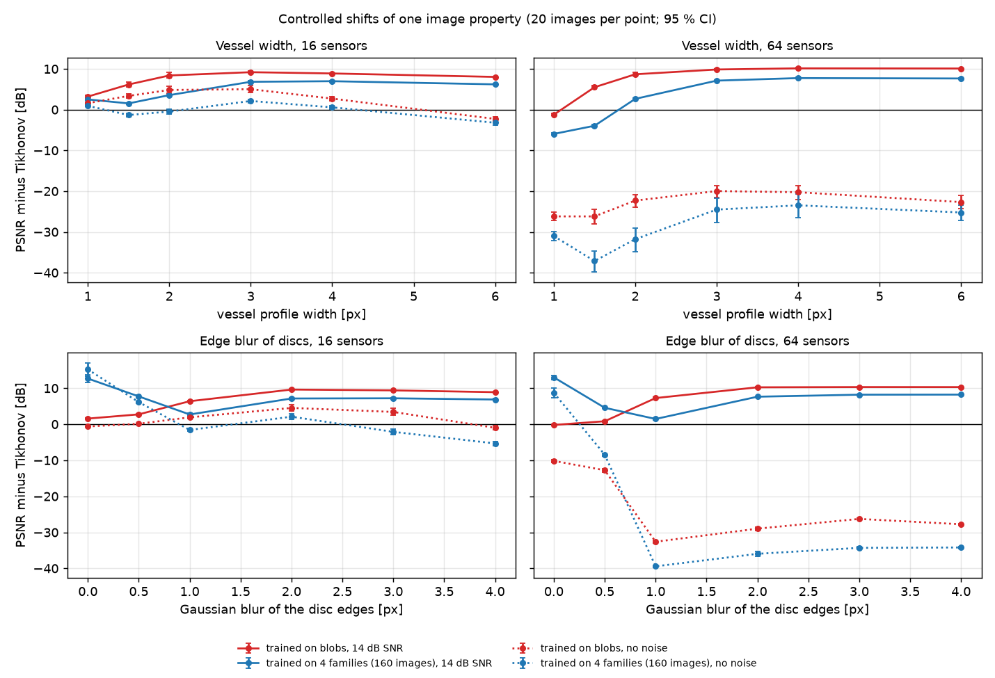
Two controlled sweeps vary one image property with everything else held fixed and nothing retrained. With 64 sensors at 14 dB SNR, the mixed network moves from 6.0 dB behind Tikhonov on vessels one pixel wide to 7.7 dB ahead on vessels four or more pixels wide, so the vessel failure is one of thin structures. The disc edge-blur sweep is non-monotonic: the mixed network's advantage falls from 13 dB on sharp discs to 1.5 to 2.7 dB at one pixel of blur, then recovers to 7 to 8 dB for smoother edges. The prediction that it would keep its advantage under blur was wrong.

A Mahalanobis distance from the training images, built on seven structural image statistics, correlates with the loss of advantage when families are pooled (Spearman −0.60 and −0.66 for the mixed networks at 14 dB SNR), but within a family it has no consistent sign and it rates the half-blurred discs as close to the training set. It ranks families; it is not a reliable per-image failure detector.

PSNR advantage over Tikhonov against vessel width and against disc edge blur, for blob-trained and mixed-trained unrolled networks at 16 and 64 sensors, with and without noise — Controlled shifts: PSNR advantage over Tikhonov against vessel width (top) and against Gaussian blur of disc edges (bottom). 20 images per point, 95% intervals. Select figure to enlarge.

Preregistered edge-sharpness intervention

One explanation of the blur valley, formed after the sweep was seen, was that the mixed training set contains one-pixel edges and smooth blob profiles but nothing in between. The intervention tested it by replacing half of the sharp-edged training images with copies whose edges are blurred by 0.25 to 1.5 pixels, at constant training-set size, and changing nothing else. Five networks were trained against the five existing controls.

The preset criteria were met with both sensor counts. At 14 dB SNR the worst advantage over Tikhonov in the valley rose from 2.7 to 8.7 dB with 16 sensors and from 1.5 to 7.0 dB with 64, at a cost of 0.5 to 1.1 dB on sharp shapes. Thin vessels, which no network was trained on, improved by 3.3 and 3.9 dB on the two thinnest widths. This supports the missing intermediate edge regime as a major cause of the valley. It did not remove the vessel failure: lines one pixel wide remained 4.0 dB behind Tikhonov with 64 sensors.

Preregistered thin-structure diagnostic

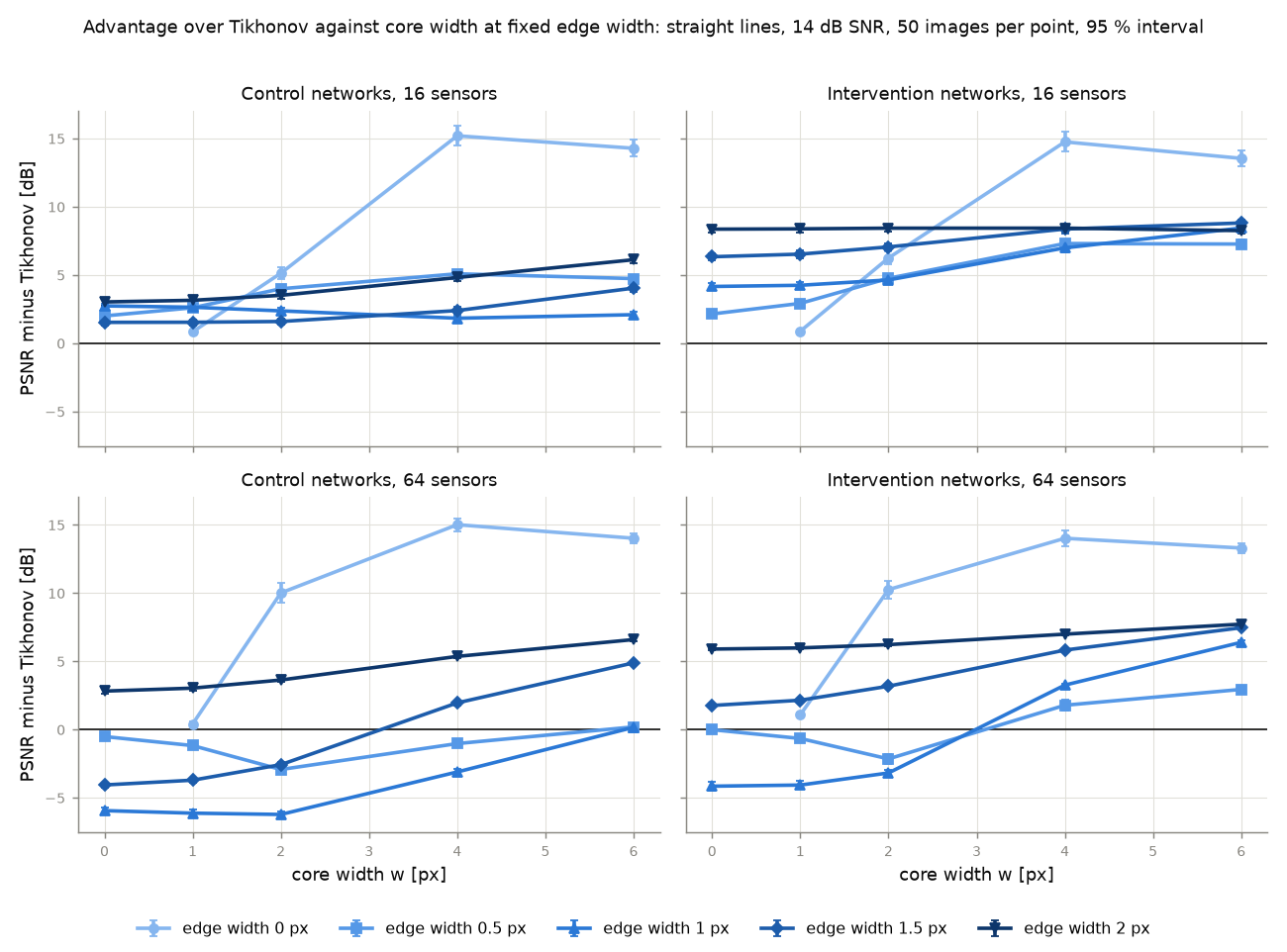
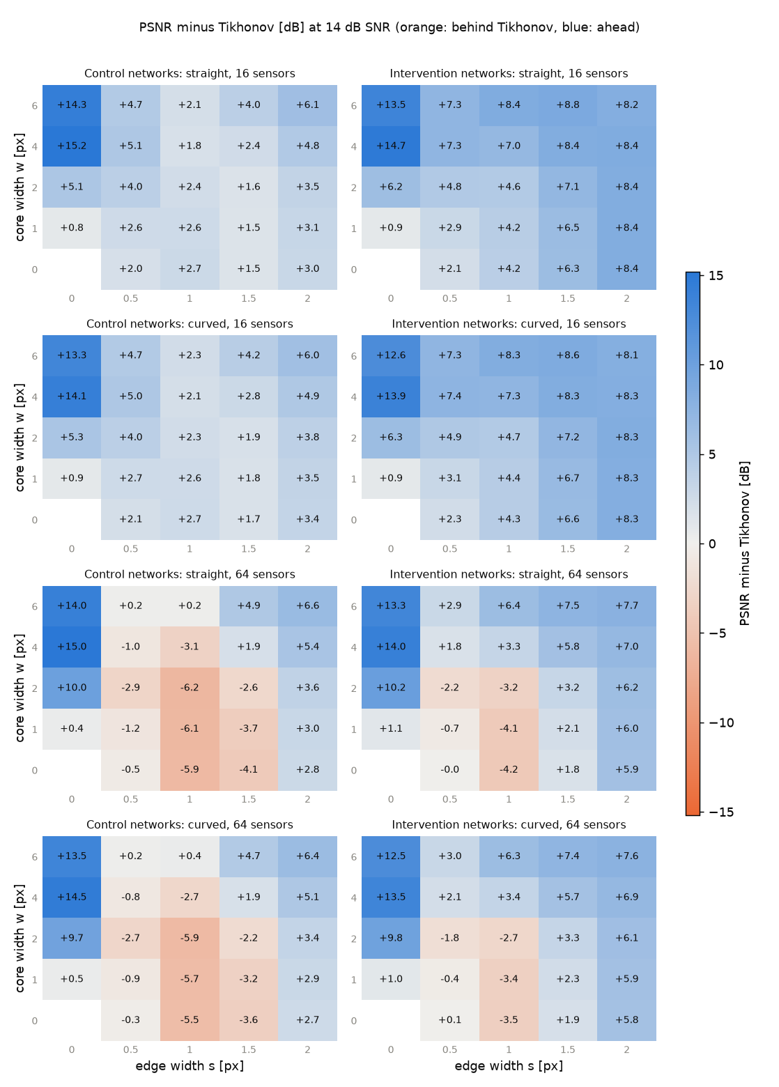
In the vessel sweep, one number set both the thickness of a line and the sharpness of its edges, and every line was curved. A factorial test set separates the three properties as far as a 64 × 64 grid permits: lines with a flat core of chosen width and a Gaussian edge of chosen width, on a straight or a curved centreline. The ten existing networks and Tikhonov were evaluated on 48 cells (5 core widths, 5 edge widths, 2 geometries) at 14 dB SNR, with 50 independent images per cell and the same phantoms for both sensor counts. No network was trained. The advantage A below is the PSNR of the five intervention networks minus that of Tikhonov, with 95% intervals over images.

−3.46 dBThinnest curved line vs. Tikhonov, 64 sensors [−3.69, −3.23]: the residual failure, reproduced

+10.54 dBWidth contrast at fixed edge width, 6 px line minus thinnest line [10.24, 10.85]

−0.70 dBStraight minus curved at the thinnest profile [−1.06, −0.32]

+12.58 dBSharp bars of trained width minus a 1 px sharp bar [12.12, 13.03]

The residual failure was reproduced. On the thinnest curved line with 64 sensors, Tikhonov reaches 36.42 dB and the networks 32.97 dB. The earlier sweep had given −3.96 dB on 20 other images.

Structural thinness was supported. At a fixed edge width of one pixel, a line 6 pixels wide is 10.54 dB better relative to Tikhonov than the thinnest line, in all five networks and on straight and curved lines alike. Of that difference, 6.69 dB is the networks scoring higher on the wide line and 3.85 dB is Tikhonov scoring lower on it, so part of the effect is the classical method doing well on thin lines.

Curvature was not supported as a cause. Curved lines were slightly better than straight ones at every thin profile tested, by 0.2 to 0.7 dB.

Sharp thin bars also lose the advantage. A sharp-edged bar one pixel wide is 1.07 dB ahead of Tikhonov, against 13 to 14 dB for bars 4 and 6 pixels wide, whose widths lie inside the training range.

The edge-profile positive control was not reproduced with 64 sensors. On bars 6 pixels wide the control networks showed the expected dip (6.43 dB), and the intervention improved the one-pixel edge by 6.23 dB [6.01, 6.44], but the preset valley-gain criterion came out at 2.78 dB against a required 3 dB. Edge profile remained influential descriptively, but its preregistered positive control narrowly missed the confirmation threshold, so the edge-axis interpretation was left unvalidated.

No interaction between factors reached the preset flag with 64 sensors. The preset rule returned the classification mixed: thinness, edge profile (edge axis not validated: H2 not reproduced). In plain terms: structural thinness was the best-supported remaining factor, curvature was not supported as a cause, and the relative contribution of edge profile remained unresolved.

PSNR advantage over Tikhonov against the core width of straight lines at five fixed edge widths, for the control and intervention networks with 16 and 64 sensors at 14 dB SNR; with 64 sensors the advantage is negative for narrow soft lines and rises with width, with 16 sensors it is positive everywhere — Advantage over Tikhonov against core width at fixed edge width, straight lines, 14 dB SNR. Rows: 16 and 64 sensors. Columns: control and intervention networks. 50 images per point, 95% intervals. Select figure to enlarge.

Sensor count

With 16 sensors, both network groups stayed ahead of Tikhonov in every one of the 48 cells. The residual failure was not reproduced there, and by the preset rule no classification was drawn (failure not reproduced: no classification). With 64 sensors, a compact failure region appeared for narrow soft structures: edge widths up to one pixel and core widths up to two. The same networks reconstruct the same thin lines acceptably relative to Tikhonov when measurements are sparse, so the failure is not simply that the network cannot represent thin structures.

Interpretation, not an established mechanism: the failure appeared only where the classical inversion benefited most from the denser 64-sensor measurements, which suggests an interaction between the behaviour of the learned prior and the information in the measurements rather than a purely geometric failure. This was not tested.

Maps of PSNR advantage over Tikhonov at 14 dB SNR over core width and edge width, for the control and intervention networks, straight and curved lines, 16 and 64 sensors; all cells are positive with 16 sensors, and with 64 sensors a group of cells at small core width and edge widths of 0.5 to 1.5 pixels is negative — The full factorial response: advantage over Tikhonov in dB for every core width and edge width, by network group, geometry and sensor count. One symmetric colour scale; orange is behind Tikhonov. Select figure to enlarge.

Limitations

Everything is synthetic: a simulated forward model and synthetic phantoms on a 64 × 64 grid, two sensor counts, one simulator, i.i.d. Gaussian noise, and one mismatch type (sound speed). Nothing was validated on measured data. Tikhonov inverts the operator that generated the data, and its weight uses the known test noise level. Each point of the two earlier controlled sweeps is 20 images per sensor count.

In the thin-structure diagnostic, width and edge profile cannot be perfectly separated near one pixel on this grid. The primary thinness contrast compares a narrow Gaussian ridge with a flat-topped bar, which differ in slope and shape as well as in width, so it retains residual confounding. In the region where the two parameters are cleanly separable, the width effect is smaller, about 3.1 dB. The edge-profile positive control was not reproduced with 64 sensors. On the 41-image subset excluding very short lines, the preregistered classification changes because the geometry criterion becomes negligible, which shows that the summary classification is sensitive to this subset choice; the primary verdicts on thinness (H1), the edge-profile control (H2) and sharp thin bars (H4) remain unchanged. Thinness has therefore not been established as the sole cause, and no follow-up training intervention was performed. The results characterise this setup, not photoacoustic reconstruction in general.

PSNR of calibrated time-reversal, the U-Net and Tikhonov at 16 and 64 sensors, noiseless and at 14 dB SNR, as the true sound speed departs from the assumed value by 0, 1 and 2 percent; Tikhonov collapses on noiseless data under mismatch and keeps a shrinking lead at 14 dB SNR — PSNR under sound-speed mismatch on 400 test images: every method assumes 1500 m/s while the data use 1500, 1515 or 1530 m/s. Shaded band: range of the 5 trained U-Nets; off-axis values are labelled. Select figure to enlarge.

Code →

Reproducibility

Source code, implementation details and available experiment records are linked in the project repository. The stated findings are specific to the documented evaluation setup.

← Back to project index